PDF:

---

Context: It is hypothesized that a fifth force of nature can be observed as interplanetary interactions. Here, we look at how planet ‘s zonal wind profile may be affected by this force from by way of instantaneous velocity boosts every according to when distance is less than distance, where is a major solar system body whose mass is significantly greater than ; C is some positive constant; is ‘s latitude from ; and are ‘s sidereal rotation period and mass, respectively; and , , and are unit vectors representing ’s north celestial pole, ’s north celestial pole, and ‘s position from , respectively. A full description can be found here: Mathematical Model Used to Predict Interplanetary Phenomena

---

Hypothesis

We test the idea that there is a connection between U(m) and U-winds for each planet with an atmosphere. In particular, if U(m) is positive, then the U component of our hypothesized velocity vector points in the eastward direction. For convenience, call this vector U, where U(m) is its magnitude. Therefore, equatorial winds should generally be in the same direction as U [figure 1].

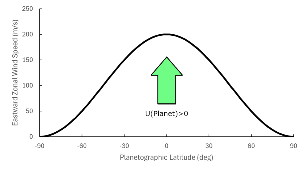
Figure 1: Positive U(m) causing eastward winds.

Conversely, if U(m) is negative, then U points in the westward direction. Therefore, equatorial winds should generally be in that direction [figure 2].

Figure 2: Negative U(m) causing westward winds.

Venus

Figure 3, adapted from Sánchez-Lavega et al (2023) shows Venus’s zonal wind velocities at different latitudes, based on cloud-tracking data collected at UV and infrared wavelengths (65-70 km and ~60 km altitudes, respectively) [Ref 1]. The wind direction is westward at all latitudes with no appreciable differences between equatorial and mid-latitude velocities.

Figure 3: Meridional profiles of the zonal wind velocity on Venus. Adapted from Sánchez-Lavega et al, 2023, The Astronomy and Astrophysics Review. This data was gathered from multiple space missions, including Mariner 10, Pioneer-Venus, Galileo, and Venus Express. The red lines represent UV data, while the blue lines show infrared data. The red arrow represents the average long-term direction of U.

Figure 4 shows that over time, U(Mars) has a net negative value (, pushing with Venus’s prevailing wind). As well as being in agreement with our hypothesis, it may be the case that U(Mars) at least contributes towards the overall super-rotation of the planet’s zonal winds.

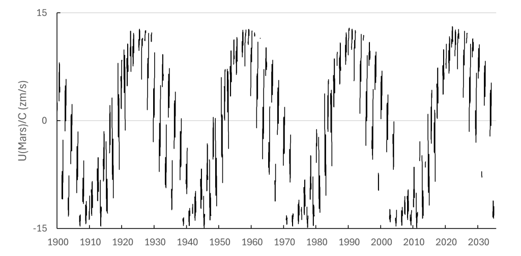
Figure 4: U(Mars) applied to Venus 1900-2035.

In a separate blog post, we’ve also included evidence of a correlation between short-term variability of wind speeds (1978-present) and U(Mars) [Ref2].

Earth

Figure 5a shows long-term zonal wind profiles on Earth together with latitudinal positions of Mars (from Earth) for each month. The equatorial dip in velocities appear to follow Mars’ latitudinal position. An animation of this (figure 5b) shows the atmosphere appearing to respond to Mars’ long-term latitudinal movements. Figure 6 confirms that over time, U(Mars) has a net negative value (pushing against Earth’s prograde winds). This is also in agreement with our hypothesis. Evidence of a connection between short-term wind speeds (1981-2024) and U(Mars) is included in a separate blog post [Ref3].

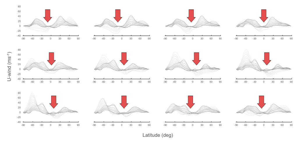
Figure 5a: Mars’s long-term latitudinal position and Earth’s zonal wind profile. Red arrows represent Mars’s long-term (1991-2020) latitude for the first of each month. Thin lines represent long-term (1991-2020) U-wind speeds at each pressure level. Months are shown chronologically from left to right, top to bottom.

Figure 5b. Animation of Mars’s long-term latitudinal position and Earth’s zonal wind profile.

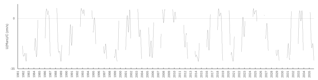
Figure 6: U(Mars) applied to Earth 1981-2035.

Jupiter

Jupiter’s zonal wind profile (figure 7) shows variability over each latitude including a mixture of prograde and retrograde flows. Figure 8 shows that over time (1750-present), U(Uranus) has also varied between positive and negative. While it is difficult to form a conclusion from the long-term picture, there is a possible connection over the short term (2009-present) [Ref 4]. This will also be included in a separate blog post.

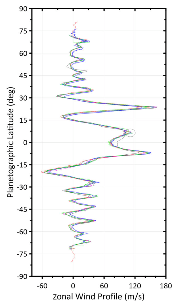
Figure 7. Jupiter’s zonal wind profile (adapted from Sánchez-Lavega et al, 2023).

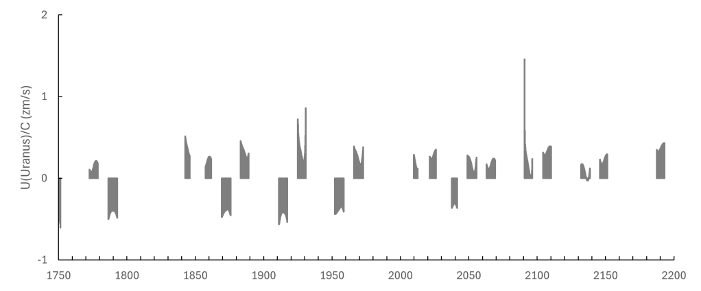
Figure 8: U(Uranus) applied to Jupiter 1750-2200.

Saturn

Figure 9 shows that Saturn has prograde (eastward) equatorial wind speeds. Also, figure 10 shows that U(Uranus) has been consistently positive for centuries. This means that U has been pointing in the same direction as Saturn’s equatorial winds. The exception to this was during the period 1979-1991 when U(Uranus) was negative. It was expected, then, that wind speeds during this period should have slowed down. Sánchez-Lavega et al (2003) indeed found a large decrease in Hubble’s measurements of Saturn’s equatorial jet during 1996-2002 compared to Voyager’s measurements during 1980-81 [Ref 5]. The next period where we should see significant values of U(Uranus) is December 2025 to June 2037. Figure 10 shows that U(Uranus) will have a similar magnitide to the last one, and also in the retrograde direction. It is natural, therefore, to predict that Saturn’s equatorial jet will undergo a slowdown of a similar magnitude.

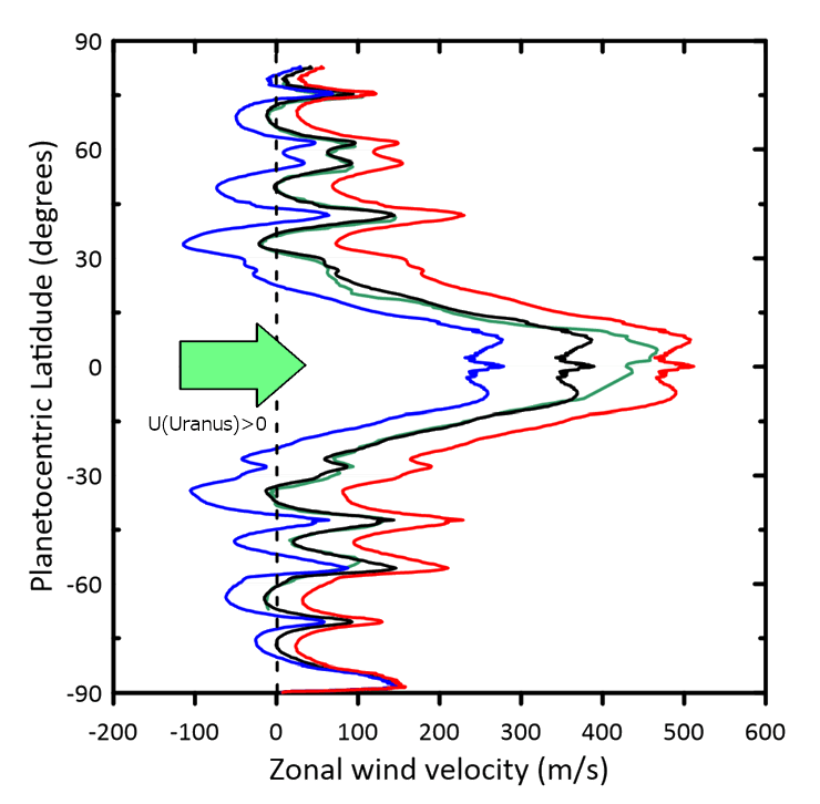
Figure 9: Saturn’s zonal wind profile (adapted from Sánchez-Lavega et al, 2023). Green arrow represents the average long-term (1750-present) direction of U.

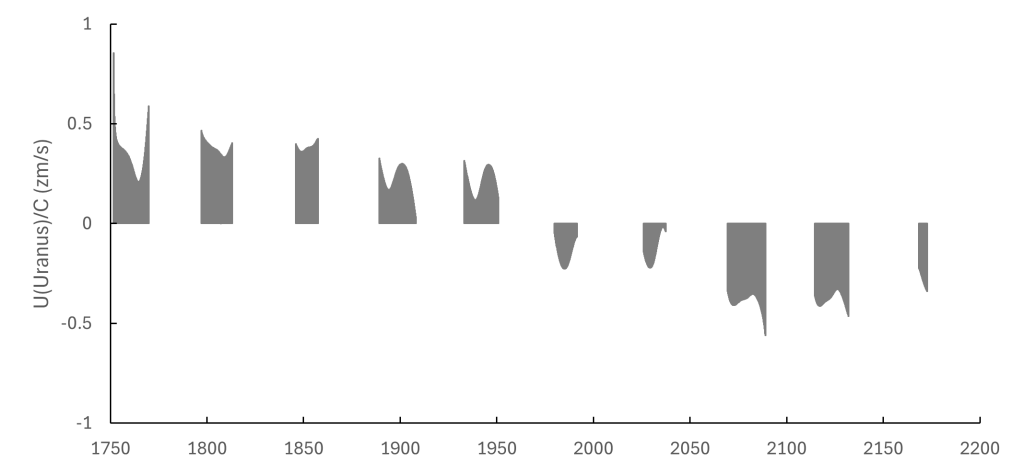
Figure 10: U(Uranus) applied to Saturn 1750-2200.

Uranus

According to our model, the greatest effect on Uranus would come from Neptune. Recalling that Uranus has a retrograde rotation, figure 11 shows that Uranus’ zonal winds are prograde (westward) at high latitudes and retrograde (eastward) at the equator. Figure 12 shows long-term (1750-2200) positive U(Neptune) with Neptune at varying northerly latitudes over Uranus. During the last period (1974-2017), this latitude averaged 57 degrees, which is indicated by the position of the green arrow in figure 11. At this latitude, Uranus’ zonal winds are maximally positive in the westward direction (and in the opposite direction to U), whereas the equatorial winds are retrograde (same direction as U), which lends extra support for our hypothesis.

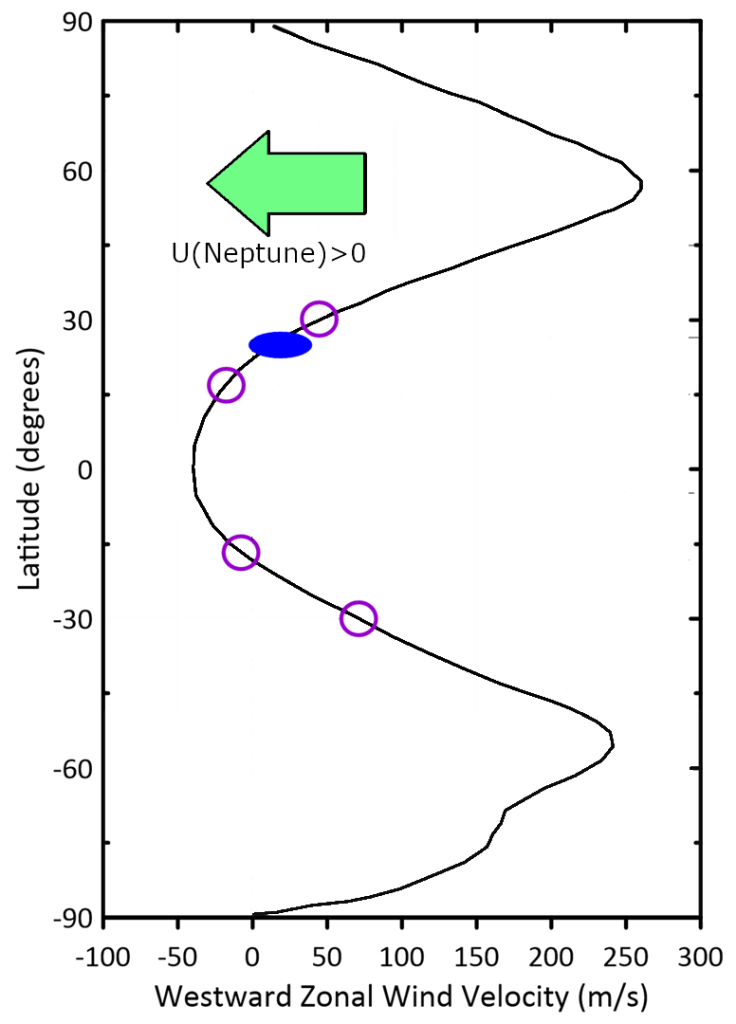
Figure 11: Uranus’ zonal wind profile (adapted from Sánchez-Lavega et al, 2023). Green arrow indicates that during the period 1974-2017, U(Neptune) was positive, with Neptune’s latitude from Uranus averaging 57 degrees north.

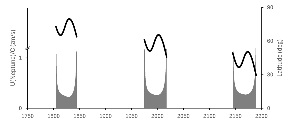
Figure 12: U(Neptune) applied to Uranus 1750-2200. Grey areas represent U(Neptune). Black lines represent Neptune’s latitude from Uranus.

Neptune

According to our model, the greatest effect on Neptune would come from Uranus. Recalling that Neptune’s rotation is prograde, figure 13 shows that Neptune’s zonal winds are prograde (eastwards) at high latitudes and retrograde (westwards) at the equator. Figure 14 shows long-term (1750-2200) negative U(Uranus) with Uranus within the latitudinal range of 20-30 degrees south over Neptune. During the last period (1977-2016), this latitude averaged 25 degrees south, which is indicated by the position of the red arrow in figure 13. With westward directions of U and equatorial winds, this also lends support for our hypothesis.

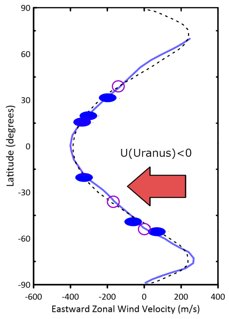
Figure 13: Neptune’s zonal wind profile (adapted from Sánchez-Lavega et al, 2023). Red arrow indicates that during the period 1977-2016, U(Uranus) was negative, with Uranus’ latitude from Neptune averaging 25 degrees south.

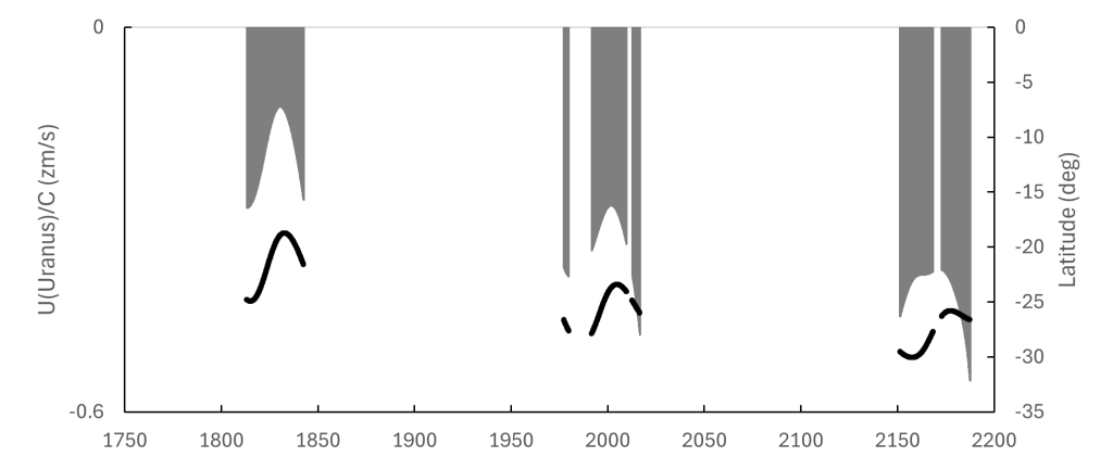
Figure 14: U(Uranus) applied to Neptune 1750-2200. Grey areas represent U(Uranus). Black lines represent Uranus’ latitude from Neptune.

References

1. Sánchez-Lavega et al (2023). Dynamics and clouds in planetary atmospheres from telescopic observations. The Astronomy and Astrophysics Review, 31(1), 5.
2. Talbot, L (2024). Evidence of Interplanetary Forces: Mars’ Influence on Venus
3. Talbot, L (2024). Uncovering Interplanetary Forces: Mars and Earth
4. Talbot, L (2024). Exploring Intermediary Forces: A Model-Based Approach to Addressing the Hierarchy Problem. Figshare preprint
5. Sánchez-Lavega et al. A strong decrease in Saturn’s equatorial jet at cloud level. Nature 423, 623–625 (2003).